The OPAL Discussion Forum

["Finn O'Shea" <finn.oshea AT nusano.com>]

Hi Andreas and Jochem,

Thank you for the responses.  I'm working off version 2.2.1.  When I run Opal it tells me I'm working with git rev. 15682d1f6008325ae35aca4ef9af14627f50a035, if that helps.

Looking at the section in Dr. Rizzoglio's thesis, I realized I was doing something foolish when computing the dispersion that was getting me close enough to suspect something strange in the code.  After reading the recommended section, (for my own future reference) I'm using cov(x,d) / var(d), where d is delta_p / p0, and it appears to produce the correct result for the dispersion:

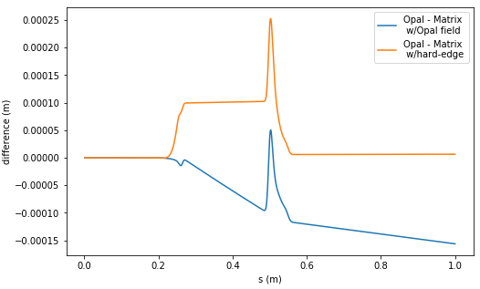
The initial dispersion of the beam is a little bit larger (more negative) than before at -0.00908 m.  But when I account for this in the formulas for dispersion I am familiar with, I get good agreement.  I also introduced some monitors, as you suggest, and found that I get slightly worse agreement at 0.55 m. The difference between Opal and treating each step as a matrix using the field in Opal and the straightforward hard-edge matrix calculation is shown in the following plot:

I'd guess the difference at 0.55 m is due to t- versus s- difference that you mentioned because the difference is constant in the body of the bend and doing stranger things in the fringes where the beam spans regions of different field strength.  The every-step-is-a-matrix method I made up does pretty good, too, but results in a slow divergence.  At any rate, I'm pretty happy with my understanding of what Opal is doing now, but I still don't understand why the beam should start with non-zero dispersion. That is a different part of the code that I haven't had a chance to look at.

Thanks again for your help,

Finn

On Fri, May 29, 2020 at 6:27 AM Adelmann Andreas (PSI) <andreas.adelmann AT psi.ch> wrote:

Dear Finn thank you again for the thoroughly analysis. Without 

such feedback, an open-source project will not survive! I (we) very much

appreciate your efforts. 

D_x in the stat file is indeed moments_m(0,5) i.r. the beam dispersion, but you 

talking about the geometrical dispersion (given by only bend properties) 

I will initiate a change request to fix the naming and documentation. 

Let me also point out that OPAL-t is integrating in time and one has do be

careful when comparing to an s-based code. The right way would be computing

all quantities at a monitor sitting at a fixed s-position and then do a post processing. 

Depending on the bunch parameters and the time step dT you have chosen the s-based

and t-based results can be different.  

Now coming back to the dispersion: 

Valeria Rizzoglio is describing in her thesis a way to calculate the geometrical

dispersion function in chapter 5.2.1 (https://www.research-collection.ethz.ch/handle/20.500.11850/280874) 

Tracking of the dispersion function. I asked her to provide the input file, which I will share

when receiving. I will make that available in the documentation. 

Please let me know your thoughts! 

Cheers A

------
Dr. sc. math. Andreas (Andy) Adelmann
Head a.i. Labor for Scientific Computing and Modelling 
Paul Scherrer Institut OHSA/ CH-5232 Villigen PSI
Phone Office: xx41 56 310 42 33 Fax: xx41 56 310 31 91
Zoom ID: 470-582-4086 Password: AdA
-------------------------------------------------------
Friday: ETH HPK G 28   +41 44 633 3076
============================================
The more exotic, the more abstract the knowledge, 
the more profound will be its consequences.
Leon Lederman 
============================================

On 29 May 2020, at 02:12, Finn O'Shea <finn.oshea AT nusano.com> wrote:

Apologies for the back-to-back emails.  Gmail appears to have stripped out all of the images and attachments.  I have included them here, I hope.

Finn

On Thu, May 28, 2020 at 5:06 PM Finn O'Shea <finn.oshea AT nusano.com> wrote:

I'm trying to understand the dynamics in bends in Opal-t and I'm seeing something I don't understand about the dispersion.  I've put together a minimum functioning examples that is a single bend (bend.in, attached).

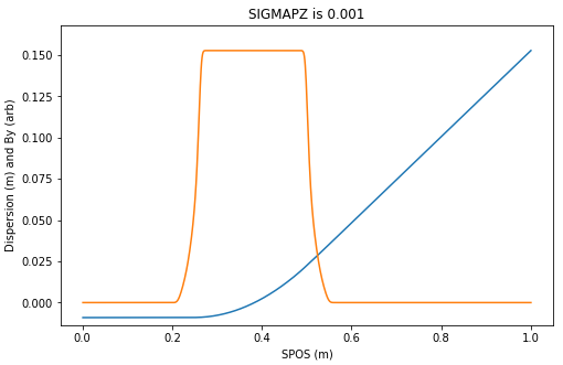
The only thing I have changed in the following examples is SIGMAPZ:

(I had to remove these inline images to get under the 1 MB email limit.)

SIGMAPZ = 1E-3 : sigma_pz_is_0p001.jpg

SIGMAPZ = 1E-2 :  sigma_pz_is_0p01.jpg

SIGMAPZ = 1E-1  :  sigma_pz_is_0p1.jpg

SIGMAPZ = 1  :  sigma_pz_is_1p0.jpg


The last one is the only image that qualitatively makes sense to me.  When SIGMAPZ is small, the dispersion doesn't change in the body of the bends at all, but it does change in the fringe field regions.

In addition, the value of the dispersion doesn't seem right to me.  For a single bend of 15 degrees and bend radius 1 m, the dispersion should end up being about 3.4 cm, but it appears to be far larger than that when SIGMAPZ is 1.  When I dig through the code to see how this value is computed, it looks like that the x-dispersion is being calculated as the correlation between x and pz/mc.  I tracked the computation down to PartBunchBase.hpp which simply returns Dx_m on line 1169.  On line 1273 it computes Dx_m as moments_m(0,5), which is simply the correlation of x and pz (I think, see line 1994).  That is not the definition of dispersion that I expected, but that could be a convention I'm unfamiliar with, is that intentional?

To check to see if the dispersion I am familiar with is doing what I expect, I dumped the bunch information every 10 steps and computed <x*d> where d = (p - p_avg) / p_avg (not pz, I compute p from px, py and pz) and I see the following evolution:

Several things stand out to me:
(1) The beam starts with a non-zero dispersion of -3.2 mm.  Why?
(2) The total dispersion "generated" by the 15-degree bend seems too small (I use SPOS = 0.55 m as the end of the magnet).  A hard-edge 15-degree magnet should have eta_f = 3.4 cm, while for this magnet it is 1.34 cm.  If I compute the dispersion using the matrix multiplication formulas I'm accustomed to (from Klaus Wille's book) I get the dispersion as 4.69 cm using the vertical field from the h5 file and treating each step as a small bend or drift.

After seeing all of this, I plotted the evolution of the beam size (not the dispersion, I dunno what is going on there already) and compared it to elegant.  This is a different lattice than above, but there is some neat stuff happening here, too.

(rms_x,rms_y,rms_s,element_names, and By_ref are from Opal, sigma_{x,y} are from elegant.  Ignore the plot after 4 meters, the lattices are different.)
 The beam sizes start off a little different because they are defined differently, and they evolve a little bit differently in the subsequent quadrupoles, but I'm more-or-less ok with these differences.  When the beam gets to the Opal dipole, rms_x starts diverging from the elegant curves pretty dramatically while y_rms seems to be doing fine.

The combination of the beam size differences (between elegant and Opal) and the dispersion differences (between Opal and other formulas) makes me think that something funny is going on in the SBEND element.  But it is possible, likely even, that I am simply unfamiliar with the conventions being used and the two can be reconciled.

Thanks in advance for any assistance,

Finn

--

Senior Scientist

Nusano, Inc

28575 Livingston Ave

Valencia, CA 91355

Office: 1 (424) 293-3174

--

Senior Scientist

Nusano, Inc

28575 Livingston Ave

Valencia, CA 91355

Office: 1 (424) 293-3174

<sigma_pz_is_0p001.jpg><mdl0.jpg><sigma_pz_is_0p1.jpg><sigma_pz_is_0p01.jpg><sigma_pz_is_1p0.jpg><bend.in><dispersion.jpg>

--

Senior Scientist

Nusano, Inc

28575 Livingston Ave

Valencia, CA 91355

Office: 1 (424) 293-3174